Imagine having a dataset of over 50 TB of compressed geospatial point data stored in flat files, and you want to efficiently filter data in a few ZIP codes for further processing. You can’t even open a dataset that large on a single machine using tools like pandas, so what is the best way to accomplish the filtering? This is exactly the problem one of our clients recently faced.
We addressed this challenge by spatially sorting the data, storing it in a partitionable binary file format, and parallelizing spatial filtering of the data all while using only open source tools within the PyData ecosystem on a commercial cloud platform. This white paper documents the potential solutions that we considered to address our client’s needs.
Figure 1: Filtering spatial data typically requires a large database to find only a few results.
Credits: NASA Earth Observatory images by Joshua Stevens, using Suomi NPP VIIRS data from Miguel Román, NASA’s Goddard Space Flight Center
Our client was a small startup who needed to avoid large up-front infrastructure costs. This constrained our approaches to those possible via cloud providers like AWS, Azure, or Google Cloud Platform (GCP). We considered five potential approaches to meet the client’s needs, one of which employs a relational database, and four that use the PyData stack.
Perhaps the first approach that comes to mind is the use of a relational database such as PostgreSQL and an extension like PostGIS which allows the use of spatial data types and queries on AWS Relational Database Service (RDS). The advantage of this approach is that it’s well established, but the strong disadvantage is cost.
Databases hosted on AWS RDS have a variety of costs, but in this case, with such a large amount of data, database storage costs dominate. Using RDS requires using more expensive database storage rather than using S3 storage. Table 1 below compares the costs of RDS Database Storage and S3 Storage at the time of writing.
| RDS Database | S3 | |
|---|---|---|
| Per GB-Month | $0.115 | $0.023 |
| Per 50 TB-Month | $5,750 | $1,150 |
Database storage is 5x the cost of S3 storage making an RDS database approach unattractive. Approaches that allow the data to be accessed directly from S3 are more cost effective. This cost difference led us to consider the PyData stack.
In this approach, building a solution using open-source libraries is more cost effective and transparent, but it’s more than that for us at Quansight. We are experts in the PyData open source tool stack. Many core contributors and creators of popular Python open source packages have found a home at Quansight. We often see solutions that make significant use of open source tools, so naturally this is where we focused the remainder of our development.
Various open source Python packages exist which could be combined to accomplish spatial sorting. We built several solutions and compared their performances below. Generally, each solution consists of five components, which are illustrated in Figure 2.
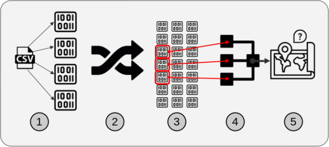
Figure 2: Illustration of the general workflow for solutions based on the PyData stack approach.
The five components are:
We chose these components generally to reduce memory use and increase filtering speed. The first component, a partitionable binary file format, was useful because partitions allow for subsets of the data to be read. The second component was spatial sorting. This is the process of mapping 2-dimensional data to a single dimension such that points near each other in the single dimension are near each other in the original 2-dimensions, and then sorting the data by that single dimension. The third component, creating a global index of the partitions, allows for efficient lookup of the partitions which contain data in a particular region. After the data was sorted and indexed, it was saved in partitions, which could be opened individually instead of opening the entire dataset at once. With the data in that format, filtering (by ZIP code polygons in this paper) was much faster because we only needed to open the data partitions relevant to a specific region. The fourth component was parallelized access and processing of the relevant partitions. The relevant partitions of the dataset include points both within and outside the set of ZIP code polygons. The fifth component, another filtering step, was necessary to exclude data outside the ZIP code polygons.
Spatial sorting deserves more explanation, and it can be performed using a variety of techniques. The idea is to map the original point data from latitude-longitude space to a 1-dimensional space such that points that are near each other in the 1-dimensional space are also near each other in latitude-longitude space. We can then sort the points based on the 1-dimensional space value. If that isn’t clear, the coming examples describing geohash and Hilbert curve spatial sorting should help.
Several established systems could be used for spatially sorting the data including Geohash, Hilbert Curve, Uber H3, and Google S2 Geometry. We only considered the first two methods due to time constraints, but they are conceptually similar to the last two methods.
Using geohashes is the first way we considered spatially sorting the point data, but what is a geohash? In practical terms, a geohash is a string of characters which represents a rectangular region in latitude-longitude space. In Figure 3, geohash “9” represents the area contained in the red rectangle. Smaller and smaller subregions can be defined within the larger geohash by adding more characters. You can see that the geohash “9q” represents the region in the light blue rectangle which is contained within geohash “9”. You can continue adding characters to the geohash to define an arbitrarily small subregion.
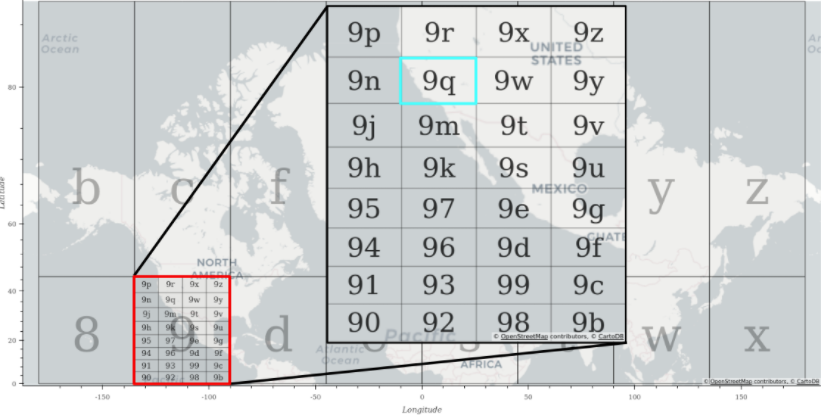
Figure 3: Background: Select one-character geohash regions plotted over a world map. Inset: All two-character geohashes starting with “9” as the first character plotted over a map.
To spatially sort the data with geohashes, we mapped each point to its four character geohash, and then sorted the geohashes lexicographically. This results in the 2D latitude-longitude space being mapped to a 1D geohash space (string of characters) which can be sorted. The power of this method depended on the fact that points near each other in geohash space are also near each other in latitude-longitude space.
Hilbert Curve Spatial Sort Example
Instead of using geohashes, the point data could be spatially sorted via a Hilbert curve. In Figure 4, the Hilbert curve (red), is a continuous curve beginning in the bottom left, and ending in the bottom right which fills the 2D latitude-longitude space. If we snap our point data, to the nearest part of the Hilbert curve, we can define each point by the distance it lies along the Hilbert curve. We can then sort the data by the 1D Hilbert curve distance. After doing so, we’ve mapped our 2D latitude-longitude data to a 1D Hilbert curve distance dimension, and points which are near each other on the Hilbert curve are also near each other in latitude-longitude space.
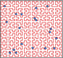
Figure 4: Image of 2D points plotted over a Hilbert curve in a latitude-longitude coordinate system. The red curvy line is the Hilbert curve inside the box. The points are arbitrary examples showing where they might lie relative to the curve.
Now that the components of the general approach have been explained, let’s get into the specific packages implemented in the four solutions we tested. We conducted performance tests on the following stacks (Table 2) to help determine the best solution for our client.
Table 2: Packages used in each spatial filtering solution.
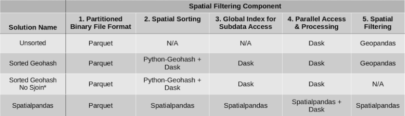
*Sorted Geohash No Sjoin is not as accurate as the other solutions.
Parquet was used in all four potential solutions as the binary file format allowing partitioning of the data for subsequently accessing only relevant data partitions. For spatial sorting, solutions using both geohashes via Python-Geohash and the Hilbert curve via Spatialpandas were considered. Dask was used to build a global index of the data in the geohash sorted solutions, while Spatialpandas built the global index of the data in the Hilbert curve solution. Dask is used to read the data in parallel in all cases. Additionally, Dask is used to map the spatial filtering function across each of the data partitions in all cases. The spatial filtering function, a spatial join (explained below), was part of GeoPandas in the first 2 cases, and part of Spatialpandas in the last case. In the Sorted Geohash No Sjoin case, no final spatial filtering was performed, resulting in a lower-accuracy solution than the other cases.
The spatial filtering function used in the last step was a spatial join. A spatial join is like a regular database join, except the keys being joined are geometric objects and the relationships between them can include geometric relationships (e.g., ‘join by points within a polygon’). Different spatial join methods are implemented in GeoPandas and Spatialpandas.
In order to compare the various solutions, we established a benchmark against which to compare the solution performances in terms of runtime. The task is to filter a large amount of point data by various randomly selected US ZIP code polygons. We performed the task five times for each solution, each time increasing the number of ZIP code polygons. The dataset and machine specification details are given below. Our work can be freely downloaded and reproduced from this GitHub repository.
Each benchmarking test follows these steps:
Preprocess data (if necessary) one time:
Filter data for each query:
We used a dataset from OpenStreetMap (OSM) (direct download link), which originally consisted of 2.9 billion latitude-longitude point pairs. We removed data outside the contiguous US, leaving 114 million rows of point data in a 3.2 GB uncompressed CSV file. We then converted the data to a Parquet file format. The polygons are randomly selected US ZIP code polygons available from the US Census (direct download link, via archive.org).
Although a cloud cluster was used in production, the benchmark results presented here were performed on a workstation. The specs are included below:
Note that the final computation brings the filtered data into the main process potentially using more RAM than an individual worker has.
As a baseline, we timed an unsorted case first. In this case, preprocessing and sorting of the data was not necessary. We simply opened up every partition of the data, and used GeoPandas to spatially join each partition of points with the set of ZIP code polygons. We spatially joined the partitions in parallel with Dask. The results are in Table 3.
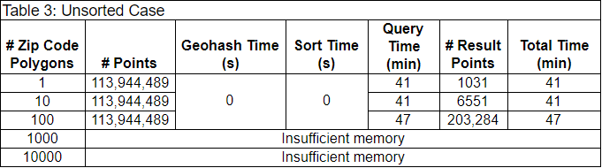
Each row contains the results of filtering the 114 million initial points by a different number of ZIP code polygons. Because this baseline does not require preprocessing, the Geohash and sort times are each 0 seconds. The query times were all above 40 minutes, and increased with increasing numbers of ZIP code polygons. The workers didn’t have enough memory to filter by 1000 or 10,000 ZIP code polygons.
The next case used Python-Geohash to create geohashes for each point in our OSM dataset. Remember that this means each point in our dataset was labeled with a string of characters representing its location. Then, Dask was used to sort and index the data by the geohash labels. The geohash calculation and sorting times are one-time costs for a given dataset of points. The remaining steps must be performed each time a query is made, and are explained with the help of Figure 6 below.
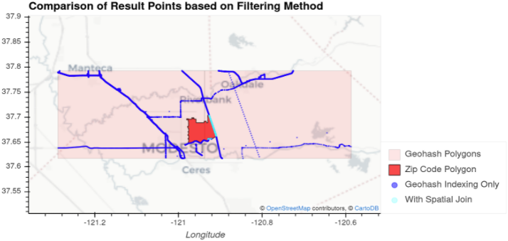
Figure 6: Illustration showing the spatial features involved in querying data in the sorted geohash case.
In Figure 6, there is a bright red region representing a ZIP code area. The light blue and dark blue points are the subset of the points from our OSM dataset that lie within the pink geohashes (two, side-by-side) which intersect the ZIP code area. Our goal was to efficiently return the light blue points, those that intersect the ZIP code area. This was accomplished by opening only the data in the geohashes (partitions) intersecting the ZIP code polygon (light and dark blue points) using the global index of our spatially sorted data, and then applying spatial filtering to leave only the light blue points.
In terms of our PyData stack, we first find the geohash polygons which intersect the ZIP code with Polygon-geohasher. Then we open our dataset with Dask. Dask uses its global index to open the partitions of our dataset corresponding to the geohash polygons (dark blue points). Then we used GeoPandas to perform a spatial join between the ZIP code polygon and the geohash points to exclude points outside of the ZIP code polygon and keep the points of interest (light blue points). The benchmark results are below.
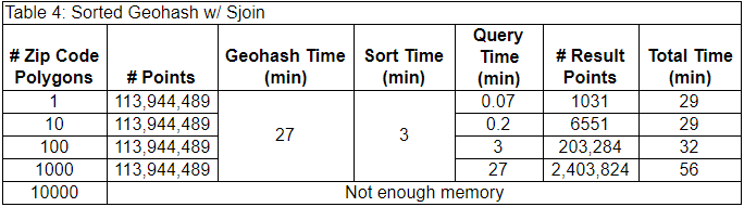
The one-time costs alone (30 min) are less than the single query time (~40 min) in the unsorted case (above), and this case was able to filter the data in the 1000 ZIP code polygon task. It’s important to note that the numbers of filtered data points are identical to the unsorted case, giving us confidence that we selected the same points.
As the number of ZIP code polygons grows, the last spatial join step takes longer and longer. For some applications, the last spatial join step may not be necessary. The lower accuracy of returning all points that are near the ZIP code polygons, rather than only those within the ZIP code polygons reduces the query time significantly. In Figure 6, this solution would return all the light and dark blue points within the geohashes intersecting the ZIP code rather than just those light blue points within the ZIP code. This solution is not adequate in all cases, but the reduced query time may be worth it in some use cases. For example, this solution may be adequate when the uncertainty of the point data is greater than the size of the geohashes. The results of leaving off the last spatial join step are below.
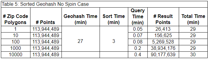
In this case, the query times are much lower, especially when the number of ZIP code polygons is higher, but the number of result points is also much larger, indicative of the lower filtering precision produced by excluding the last spatial join step.
The last case used a new package called Spatialpandas. Spatialpandas spatially sorts the data using the Hilbert curve. The results of using Spatialpandas are below. It wasn’t possible to separate the preprocessing time from the spatial sort time in this case, so they are included together in the sort time column.
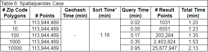
* Geohash time and sort time are combined because they could not be determined separately with Spatialpandas.
This case was much faster than the other cases. Additionally, this was the only case that could filter the data by the 10,000 polygon set with full accuracy. This is because the Spatialpandas spatial join requires less memory than the GeoPandas spatial join method.
We’ve looked at the results individually, but the following plots compare the performances of the potential solutions. The first plot below shows the query times vs the number of ZIP code polygons by which the data was being filtered. Query times don’t include the one time costs like calculating geohashes, the Hilbert curve, or sorting the data.
As shown in Figure 7, the query time for the unsorted case (red) took the longest at over 40 minutes, and this case was not able to process the two largest batches of ZIP code polygons. The query time for the sorted geohash without spatial join (yellow) was the fastest for 100 or more polygons, but remember that it wasn’t as accurate as the other solutions. The fastest query time for an accurate solution is the Spatialpandas case (green).
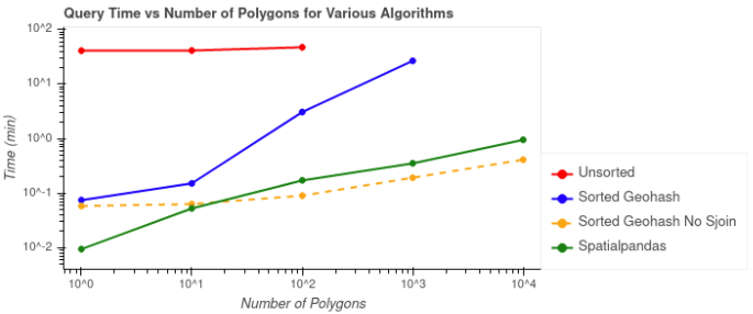
Figure 7: Comparison of filtering time for each batch of ZIP code polygons. The dashed line indicates the case in which a spatial join was not used and the results are typically less accurate.
Having looked at query times, now let’s look at the one-time preprocessing times shown in Figure 8. No preprocessing was necessary for the unsorted case, so the preprocessing time was 0 minutes. The two sorted geohash cases had the same preprocessing steps and are identical as a result. In the sorted geohash cases, the geohash calculation took 27 minutes, and the sorting took 3 minutes. By contrast, in the Spatialpandas case the preprocessing and sorting steps took just over 1 minute.
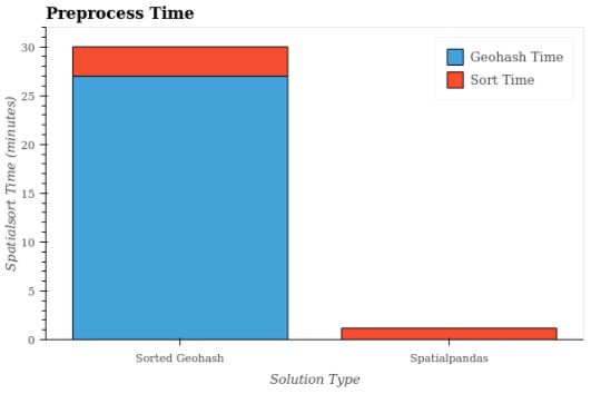
Figure 8: Preprocessing times for the Sorted Geohash and Spatialpandas solutions. For Spatialpandas, the sort time includes the preprocessing time.
Figure 9 shows the extrapolated total time (preprocessing + query time) vs the number of queries when filtering the data by 1, 100, and 10,000 polygons in each query. Query times are extrapolated under the assumption of linear scaling of queries based on the results of the single query time.
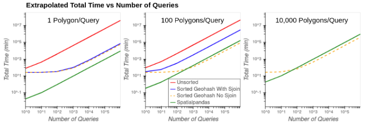
Figure 9: Extrapolated total time vs number of queries using 1 polygon (left), 100 polygons (middle), and 10,000 polygons (right) in each query.
Of the approaches with highest accuracy, the Spatialpandas solution is projected to be fastest in all situations. At times, the Sorted Geohash No Sjoin solution has lower total time than Spatialpandas, but this comes at the potentially high cost of accuracy.
Spatialpandas was the best overall solution explored here, and was what we ended up using for our client. Spatialpandas is an easy to install, pure Python package. It makes heavy use of Numba for highly efficient spatial joins and bounding box queries. It’s also integrated nicely with Dask and the Parquet file format.
However, there are additional considerations to keep in mind. Spatialpandas is a young project with a small community at the moment. The documentation is limited compared with more established libraries, and it has low development activity for the moment. Spatialpandas is good at what it does, but it’s also limited in functionality. If you need Spatialpandas to do something similar, but slightly different from what is shown here, you may be forced to implement changes to the library yourself. Keep these considerations in mind if you’re thinking of using Spatialpandas in your application.
We considered and experimented with a few other approaches. AWS Athena is a serverless interactive query service allowing users to query datasets residing in S3 via SQL queries. Though promising, at the time Athena had file size limitations that made it impractical for this use-case and also did not obviate the need to sort and partition the data spatially to improve access times. The other main area considered was GPU acceleration. We explored two technologies for this, OmniSci and NVIDIA RAPIDS. These showed some promise but turned out to be too expensive to be practical. Omnisci has excellent GPU accelerated geospatial query performance but requires a fairly beefy GPU instance to run and requires that the data be imported into its internal format, which also increases storage costs over S3. The NVIDIA RAPIDS suite has a new tool called CuSpatial, but in practice it was a very early prototype and not usable in production.
Reach out to Quansight for a free consultation by sending an email to connect@quansight.com.
This work was originally presented at SciPy 2020, and can be viewed here: