

This post is based off of a talk given at PyData NYC 2022. You can watch the talk here: Scaling Python: Bank Edition.
Often scaling a distributed computation is easy… that is, until it isn’t. There are currently several tools that will get you off the ground quickly, but when the size of your data increases and you are required to scale further, the complexity needed for a solution often increases considerably, beyond what these tools are able to handle. At this point, algorithm- and infrastructure-dependent requirements will likely preclude experimentation and problem solving. While new tools are continuously emerging that promise straightforward hyper-scaling, in most situations there are at least a few confounding details that have to be ironed out manually.
In this post, we walk you through how Quansight helped a banking client through this process of scaling Python DataFrame calculations in a real-life scenario. After exploring GPU computation and investigating a variety of approaches to in-CPU DataFrame aggregation, we found that a combination of Argo Workflows and Dask Bag provided the scalability and flexibility we needed to meet our client’s needs. Note that we’ve kept that client’s name and key details of the project anonymous for privacy reasons.
path, Date, and value. Each file contained 50,000 simulations, where the path for each simulation spanned the same set of 120 non-sequential dates into the future (resulting in 6 million rows of data per file).
Each file belonged to a particular file group, with the size of each group ranging from two to 18,000 files. Our goal was to sum the value entries in all of the files within each file group over each unique (path, Date) combination. We needed to do this very quickly to allow generation of results in as close to real time as possible. To complicate the problem, we had to be able to accomplish this while accounting for potentially limited compute resources.
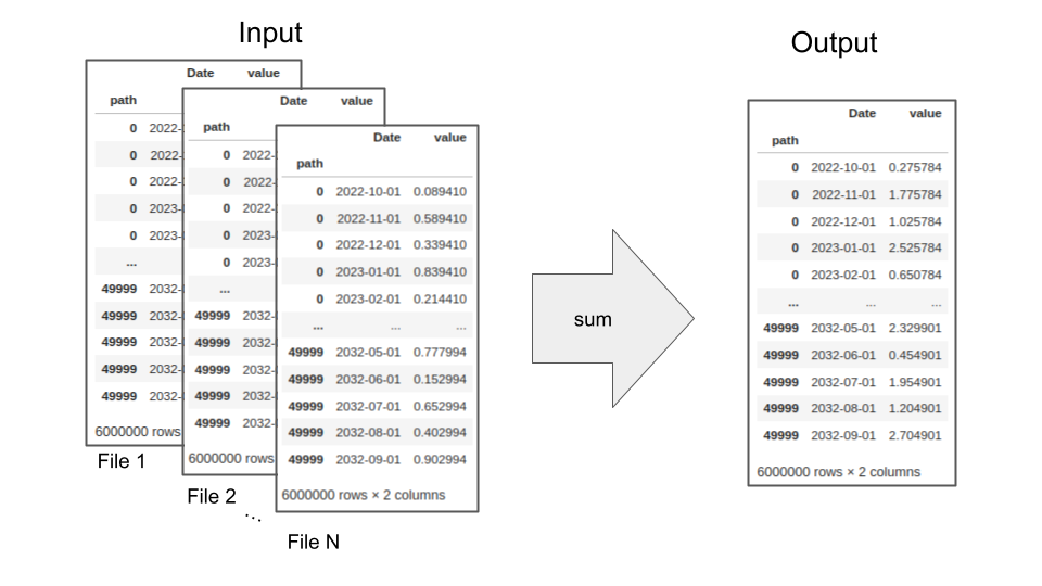
Schematic of the required summation across multiple input files.
As the first step in solving this problem, we explored the hardware options that were available to us. Specifically, as we were basically doing matrix summations on a large scale, we were curious if switching the computation to GPUs, which are highly efficient at matrix computations, could provide the performance we needed. We also thought that GPUs might be able to help us compensate for the effect of networking and other I/O bottlenecks. Finally, we thought that GPUs could help us in optimizing the memory usage of our for-loop operations. We would be able to set up our computations using n-D arrays and for-loops with striding to reduce the amount of memory used at one time.
We examined several libraries that use a GPU compute engine as their back-end. A number of these were from the RAPIDS stack. We put TensorFlow and PyTorch to the test, but found that they were not well suited to this problem due to some machine-learning specific assumptions they make under the hood. The RAPIDS stack libraries we explored were cuDF, CuPy, and blazing-SQL (though this has now been deprecated in favor of Dask SQL). Another tool that we tried was HEAVY.AI, formerly OmniSci. While HEAVY.AI was fast, it could not handle simultaneous read/write, which was a showstopper for us.
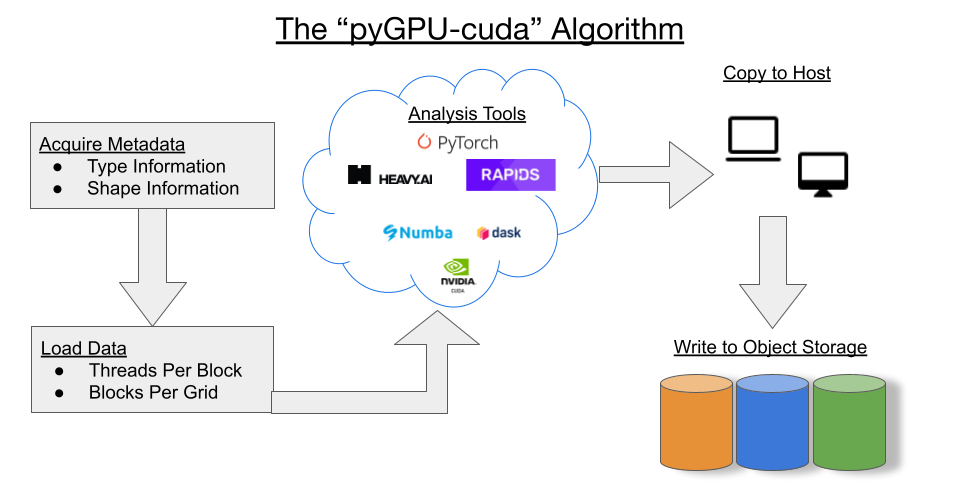
GPU architecture lends itself to a pattern that many of these tools rely on, which is exposed as the CUDA programming model. In this model, individual threads are grouped into blocks, and these blocks are clustered into grids. It is these grids that are actually executed on the GPU.
A calculation like the multi-source summation we need to do here is carried out in multiple steps. First, metadata is used to determine the maximum threads per block and blocks per grid. Then, the input data is loaded into GPU memory using this information and the computation is run using one of the above tools. Finally, the data is extracted back to the memory environment of the host. For more background on techniques for memory swapping between main RAM and GPU-RAM, see this NVIDIA blog post.
Unfortunately, we discovered that the process of copying the data back and forth between the host’s memory and the GPU memory turned out to be expensive enough to negate a lot of the benefits we saw in the speedup of the computation itself by using GPUs. On top of that, the increased cost of GPU-available cloud instances made the usage of GPUs infeasible for this project. With that in mind, we decided to forego specialized computation hardware and focus on good, old distributed CPU architecture for our computation.
With our decision made to use a distributed CPU architecture, we started looking at ways we could implement Dask to solve the problem. We chose Dask as our starting point at this stage of the project due to its native Python implementation and its utilization of standard Python APIs. This makes it easy to test code in pandas or numpy and then quickly distribute the code using Dask, with only slight changes. The first approach we tried was a simple DataFrame group-by.
We thought that the DataFrame approach made sense due to the ease of implementation: take a list of Parquet files and pass that list to the Dask DataFrame read_parquet() function. We would then run the groupby() method on the loaded DataFrame and take the sum of the resulting group-by object. Below is an example of this code and an image of the Dask dashboard after successfully running the code sample. You can see that the work has run without error across 2 workers, each of which was allocated with 2 threads.
					def build_graph(paths):
    df = dd.read_parquet(paths,
                         index=False,
                         storage_options=storage_options)
    gb = df.groupby(['path', 'Date']).sum()
    return gb


graph = build_graph(paths_5)
fut = client.compute(graph)
fut.result().info()

However, as we noted in the description of the problem, we couldn’t confidently know ahead of time the total amount of resources available within the cluster being used for any given calculation. What happens if our DataFrame ends up being larger than the capacity of the cluster assigned to process it?
As it turns out, we ran into exactly this issue with some of our larger aggregations. We were finding that when we submitted jobs, workers would be forced to pause or restart when the memory thresholds for the cluster were reached, in some cases causing the job to fail completely. The below code shows an example of this happening with a two-worker Dask cluster, where each worker has 4 GB of memory. We get a ‘killed worker’ error when trying to aggregate ten 6,000,000-row files.
					>>> graph = build_graph(paths_10)
>>> fut = client.compute(graph)
>>> fut.result().info()

2023-03-31 18:58:33,630 - distributed.worker_memory - WARNING - Worker is at 83% memory usage. Pausing worker.  Process memory: 3.33 GiB -- Worker memory limit: 4.00 GiB
2023-03-31 18:58:33,792 - distributed.worker_memory - WARNING - Worker is at 76% memory usage. Resuming worker. Process memory: 3.07 GiB -- Worker memory limit: 4.00 GiB
2023-03-31 18:58:33,893 - distributed.worker_memory - WARNING - Worker is at 89% memory usage. Pausing worker.  Process memory: 3.60 GiB -- Worker memory limit: 4.00 GiB
2023-03-31 18:58:33,934 - distributed.worker_memory - WARNING - Worker exceeded 95% memory budget. Restarting
2023-03-31 18:58:33,977 - distributed.nanny - WARNING - Restarting worker
2023-03-31 18:58:51,739 - distributed.worker_memory - WARNING - Worker is at 86% memory usage. Pausing worker.  Process memory: 3.46 GiB -- Worker memory limit: 4.00 GiB
2023-03-31 18:58:52,334 - distributed.worker_memory - WARNING - Worker exceeded 95% memory budget. Restarting
2023-03-31 18:58:52,376 - distributed.nanny - WARNING - Restarting worker
---------------------------------------------------------------------------
KilledWorker                              Traceback (most recent call last)
File <timed exec>:3

File ~/.conda/envs/bank/lib/python3.8/site-packages/distributed/client.py:283, in Future.result(self, timeout)
    281 if self.status == "error":
    282     typ, exc, tb = result
--> 283     raise exc.with_traceback(tb)
    284 elif self.status == "cancelled":
    285     raise result

KilledWorker: ("('dataframe-groupby-sum-chunk-d4e753da53a3eff842bab7cbba152105-e7aebcddb75c44615a5bb2eb1e6f9433', 82)", <WorkerState 'tcp://127.0.0.1:42571', name: 1, status: closed, memory: 0, processing: 39>)
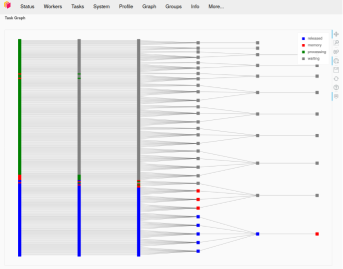
Likewise, the left pane of the Dask dashboard screenshot below shows new workers getting started after previous workers are killed. If this had run as desired, we would expect the task stream diagram to have four rows, one for each thread on each worker. Instead, we see several rows, showing new workers starting and trying to run the remaining jobs before failing. The graph in the right-hand pane shows the Dask graph for this task, demonstrating how the various summation groups are aggregated together over the course of the computation.
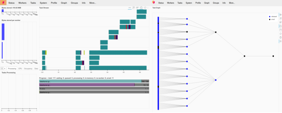
(Author’s Note: In this example, I am using an older version of Dask. This problem of workers running out of resources and being killed is becoming less of an issue as improvements to the Dask scheduler are released. In particular, I am not able to reproduce this error on the same aggregation calculation if I use a more recent version of Dask than the one available at the time we were executing this project.)
As the next step in addressing these out-of-memory errors, we used a chunking strategy. We found that if we created a graph that chunks the group-by operations into a larger number of smaller aggregations, the scheduler had an easier time handling the load.
The chunking strategy we took was as follows. For a given set of files, if the total number of files exceeded a specific threshold, we would build a Dask graph that would first load a subset of the files. Next, it would group and aggregate this subset into a single DataFrame. Then, each subsequent subset would be summed into the previously aggregated results. The resulting DataFrame would then be further grouped and aggregated as many times as required until all files were aggregated together.
In cases where there were not enough files to meet the threshold, we would follow the standard read_parquet(), groupby(), and sum() strategy described above, without any intermediate subset calculations and aggregations. This allowed us to streamline any calculations that we were confident would fit comfortably in any cluster that might be assigned to them.
The code and schematic below illustrate this chunked calculate-and-aggregate strategy for a representative large dataset.
					%%time

def build_graph(paths, batch_cutoff=10, n_per=5):
    df = None
    if len(paths) >= batch_cutoff:
        for x in range(0, len(paths), n_per):
            ps = paths[x:x+n_per]
            sub = dd.read_parquet(ps,
                                  index=False,
                                  storage_options=storage_options)
            if df is not None:
                sub = dd.concat([sub, df])
            sub = sub.groupby(['path', 'Date'])
            sub = sub.sum()
            df = sub
    else:
        df = dd.read_parquet(paths, index=False, storage_options=storage_options)
        df = df.groupby(['path', 'Date']).sum()
    return df


graph = build_graph(paths_10, batch_cutoff=5, n_per=2)
fut = client.compute(graph)
fut.result().info()
With this strategy, we were able process our largest aggregation sets when run singly, which represented a significant step forward. However, there were many aggregations to do and we wanted to run them as quickly as possible. This is where we started seeing the next set of problems. The strategy laid out so far allowed us to complete any of our aggregations on an individual basis. But when submitting thousands of aggregations at a time, where sometimes the entire job was larger than the cluster itself, we again ran into a variation of our original problem: workers were frequently running out of memory and either pausing or, worse, getting killed. This caused a lot of work to be wasted when we had to restart calculations, and sometimes led to runs erroring out completely and being unable to finish, as shown below:
					>>> [len(group) for group in small_path_groups]
[20, 15, 15, 10, 10, 10, 5, 4, 4, 2, 3, 2]
>>> graphs = []
>>> for path_group in small_path_groups:
...    graphs.append(build_graph(path_group, batch_cutoff=9, n_per=5))

>>> futs = client.compute(graphs)
>>> wait(futs)

2023-03-31 19:16:02,371 - distributed.worker_memory - WARNING - Unmanaged memory use is high. This may indicate a memory leak or the memory may not be released to the OS; see https://distributed.dask.org/en/latest/worker.html#memtrim for more information. -- Unmanaged memory: 2.62 GiB -- Worker memory limit: 4.00 GiB
2023-03-31 19:16:13,723 - distributed.worker_memory - WARNING - Unmanaged memory use is high. This may indicate a memory leak or the memory may not be released to the OS; see https://distributed.dask.org/en/latest/worker.html#memtrim for more information. -- Unmanaged memory: 2.67 GiB -- Worker memory limit: 4.00 GiB
2023-03-31 19:19:15,364 - distributed.worker_memory - WARNING - Unmanaged memory use is high. This may indicate a memory leak or the memory may not be released to the OS; see https://distributed.dask.org/en/latest/worker.html#memtrim for more information. -- Unmanaged memory: 2.77 GiB -- Worker memory limit: 4.00 GiB

 ...

2023-03-31 19:40:35,851 - distributed.worker_memory - WARNING - Unmanaged memory use is high. This may indicate a memory leak or the memory may not be released to the OS; see https://distributed.dask.org/en/latest/worker.html#memtrim for more information. -- Unmanaged memory: 2.66 GiB -- Worker memory limit: 4.00 GiB
2023-03-31 19:40:36,265 - distributed.utils_perf - WARNING - full garbage collections took 33% CPU time recently (threshold: 10%)
2023-03-31 19:40:36,384 - distributed.worker_memory - WARNING - Unmanaged memory use is high. This may indicate a memory leak or the memory may not be released to the OS; see https://distributed.dask.org/en/latest/worker.html#memtrim for more information. -- Unmanaged memory: 2.70 GiB -- Worker memory limit: 4.00 GiB
2023-03-31 19:40:38,542 - distributed.utils_perf - WARNING - full garbage collections took 20% CPU time recently (threshold: 10%)
2023-03-31 19:40:39,007 - distributed.utils_perf - WARNING - full garbage collections took 23% CPU time recently (threshold: 10%)

DoneAndNotDoneFutures(done={<Future: error, key: finalize-e92147f1de33377e5d699b9a433833ce>, <Future: error, key: finalize-84b8df9a83cf66156a75066a2ac1e76d>, <Future: finished, type: pandas.core.frame.DataFrame, key: finalize-ab97ef0c5f1a508ff7794c880dc52904>, <Future: error, type: pandas.core.frame.DataFrame, key: finalize-fa12a3d29b570a5c9fde46ad4bb4b54e>, <Future: error, key: finalize-27d9405ba12f958c13d758e631561dc1>, <Future: error, key: finalize-62c1aac7865d455c15c608feb900b359>, <Future: finished, type: pandas.core.frame.DataFrame, key: finalize-0736bf3a3c1b701cf111a7602b94688f>, <Future: finished, type: pandas.core.frame.DataFrame, key: finalize-e7a25f8b5dec897b1324baeb1058e0ae>, <Future: error, key: finalize-04ea3d501751890ece2130a20efc5dba>, <Future: error, key: finalize-d7140f09799374ca916b3cbb28816323>, <Future: error, key: finalize-89541c92fdaf68ded72329388778eadf>, <Future: error, key: finalize-0dde02417f66f47d1f389e64ee5fb966>}, not_done=set())
To combat this, we decided to throttle how much work we were going to give the scheduler at a time. To do this we employed a thread-pool executor to submit the jobs, where we spun up a fixed number of worker threads to handle the calculation workloads. This would allow us to submit many jobs at once to the calculation system, but still limit how much work was getting released to the Dask scheduler. When it reached the front of the line, each scheduled job would get a thread worker from the pool, run to completion, and then release the thread back to the pool, after which the thread-pool would grab the next job and schedule it.
However, we were still running into problems with overwhelming the cluster. One option that might work for some situations is lowering the number of thread workers, but this wasn’t helpful for us. We had some jobs that were individually larger than the cluster could handle when run in a multi-job context, even after chunking. This meant that we were still overloading the cluster when any of these large jobs were scheduled alongside some number of other jobs, and the rest of the time the cluster was significantly underutilized (a small number of threads running smaller jobs, leaving a large fraction of unused memory) making for poor efficiency and economy.
So, instead of lowering the number of thread-workers in our thread-pool, we started checking the cluster resources manually with the Dask scheduler before submitting each job to the thread pool to make sure there was enough memory to accommodate it. This strategy gave us the benefit of being able to increase the number of thread-pool workers for better cluster utilization for smaller aggregations, while also allowing us to throttle the amount of submissions when we needed more resources for larger calculations. To implement this, we set it up so that when a thread-pool worker got a new task, we would:
The code below illustrates the concept behind this approach:
					from concurrent.futures import ThreadPoolExecutor
from concurrent.futures import as_completed
from threading import Lock
from time import sleep

def build_graph(paths, batch_cutoff=10, n_per=5):
    ...
    return df

def good_to_go(needed_bytes_gb, submitted_task_cutoff=20):
    # returns is cluster has available resources
    # percent of cluster in use
    ...
    return bool, percent_use

lock = Lock()

def compute_task(graph, num_paths):
    max_size = num_paths * 200 / 1000
    go_ahead = False
    while not go_ahead:
        with lock:
            go_ahead, cluster_usage = good_to_go(max_size)
            sleep_mult = (cluster_usage * 2) ** 1.5
            if go_ahead:
                fut = client.compute(graph)
                sleep(sleep_mult)
    wait(fut)
    return fut

def creator(paths):
    n_paths = len(paths)
    graph = build_graph(paths, batch_cutoff=9, n_per=5)
    return graph, n_paths

def submit_via_threadpool(graphs):
    results = []
    with ThreadPoolExecutor(max_workers=1) as creation_executor:
        with ThreadPoolExecutor(max_workers=6) as submission_executor:
            for (graph, n_paths) in creation_executor.map(creator, small_path_groups):
                result = submission_executor.submit(compute_task, graph, n_paths)
                results.append(result)
    for fut in as_completed(results):
        print(fut.result())
    return result
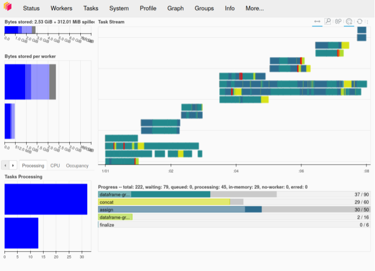
The Dask dashboard screenshot below demonstrates this strategy successfully working. We can see how different tasks are running both in parallel and consecutively as resources become available. Some begin immediately, while others wait for other calculations to finish and free their resources. This happens until all work is complete.
This strategy was starting to get us closer to a complete solution, though we still needed better performance. While we now had the ability to increase the thread-pool worker count for better cluster utilization, it was still taking a problematically long time to create the execution graphs in the first place, and we still didn’t have completely reliable calculations with our larger aggregations—computation of the execution graphs themselves would sometimes consume a problematically large amount of memory.
So, with that in mind we created a second thread-pool executor. This thread-pool was responsible for creating the Dask graphs for each aggregation group. It would then pass off each Dask graph to the next thread-pool for submission to the cluster. With the larger aggregation groups we found we could submit them via the creation thread-pool where they would throttle the amount of new graphs being created, leaving sufficient cluster resources free to run the aggregations in parallel.
With this strategy, we could reliably complete large batches of jobs, and we could do so while utilizing the cluster fairly efficiently. However there were still downsides. We were finding that tuning the thread-pool executors was tedious. It took work to figure out a suitable number of threads for each thread-pool, along with the appropriate durations for sleep calls and thread-locking. It also wasn’t a one-size-fits-all strategy, as different workloads needed different settings. All of this made for a complex setup which was far from ideal. Furthermore, the data shuffling and group-by operations continued to be undesirably expensive across a large cluster.
At this point, we started feeling like we were reaching the limits of our multi-threaded group-by strategy. It was becoming clear that our code was too complex and not very efficient. We realized that the more we continued down this path, the more technical debt we were going to accrue and the harder the project would be to manage. So we began to think of other ways we could aggregate the data.
In the course of this process, we realized that pandas (not Dask) DataFrames actually sum together quite nicely: pandas ensures that the index and columns match on the sums, so you won’t end up adding the wrong numbers together. Pandas sums are also considerably faster than group-by operations. As another bonus, moving out of Dask DataFrames would allow us to utilize multi-indexing, which helps cut down on the memory footprint of the DataFrames. We found that on our dataset, summing suitably re-indexed DataFrames was about three times faster than running a group-by operation on the equivalent concatenated DataFrame:
					>>> %timeit concated_list_of_dfs.groupby(['path', 'Date']).sum()
1.77 s ± 72.3 ms per loop (mean ± std. dev. of 7 runs, 1 loop each)
>>> %timeit sum(list_of_dfs)
639 ms ± 15.9 ms per loop (mean ± std. dev. of 7 runs, 1 loop each)
While these performance improvements were promising, we were passing a lot of data between workers causing the jobs to generally run slower, and adding extra burden to the scheduler in managing where work was. We wanted to streamline these data management aspects, and also wanted our architecture to exploit any parallelization opportunities among the different aggregation groups. Ideally, we wanted to run an aggregation group on a single worker whenever feasible, to cut down on network traffic on the cluster. With that in mind we started looking at a cluster-of-clusters approach.
We based our cluster-of-clusters implementation off of a keynote at the 2021 Dask Summit. With this setup, you have a normal Dask distributed cluster with a scheduler and a set of workers. Instead of passing your work directly to the scheduler as normal, though, you pass delayed objects that instruct the worker to start a local cluster and also to build a specific Dask graph to be passed to that local cluster. Submitting work in this way gives the benefit of being able to encapsulate a work unit in order to reduce the overall network communication needed to manage that work unit.

(K8s = Kubernetes)
However, at this point we were still using thread-pools to manage the aggregation on the local clusters, requiring the same cumbersome manual tuning as before. So, from here we decided to pivot away from the aggregation strategy to a different approach.
At this point, we started looking more seriously into Dask Bag. Dask Bag is typically used for processing text or JSON files, so it’s probably not the first thing people think of when they need to work with DataFrames. One of the big advantages of Dask Bag, though, is that it follows the map-reduce model: it allows us to take a more hands-off approach to managing the calculations because we can trust that it will reduce our data on each individual worker as much as possible before moving data between workers to finish the aggregations. When the Dask Bag object is submitted, Dask will send batches of files as defined by partition_size to the workers. The workers will then apply the mappings and the aggregation to each batch. Finally, the workers will re-partition and apply the mappings and aggregation across the newly formed batches until the dataset is fully aggregated. This helps to minimize the amount of data traveling between workers. It also let us take advantage of summing DataFrames instead of running group-by aggregations on them.
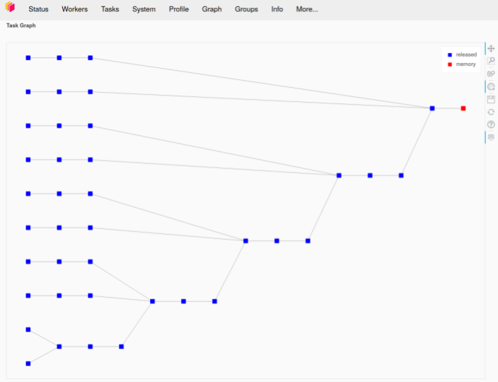
The code sample and dashboard screenshot below illustrate this approach. The screenshot shows the graph representation of several aggregation tasks that have been submitted to a Dask cluster. We can see the multiple levels of aggregation that each task goes through for each Dask Bag partition until all partitions are aggregated together. This demonstrates the map-reduce model in action.
					def load_dataframe(data):
    df = pd.read_parquet(
        data,
        storage_options=storage_options
    )
    df = df.set_index(['Date'], append=True)
    return df

@delayed
def info(df):
    buffer = io.StringIO()
    df.info(buf=buffer)
    return buffer.getvalue()

def build_task_graph(filepaths):
    part_size = 5
    with dask.annotate(resources={'MEMORY': 200*part_size}):
        b = db.from_sequence(filepaths, partition_size=part_size)
        dfs = b.map(load_dataframe)
        summed_df = dfs.sum()
    with dask.annotate(resources={'MEMORY': 200}):
        delayed_df = summed_df.to_delayed(optimize_graph=True)
    info_delayed = info(delayed_df)
    return info_delayed
In the image above is the graph representation of several aggregation tasks that have been submitted to a Dask cluster. We can see the multiple levels of aggregation that each task goes through for each bag partition until all partitions are aggregated together. This demonstrates the map reduce model in action.
On top of Dask Bag, we also started utilizing a tool called ‘resource annotations‘. These allowed us to take a much more hands-off approach to the scheduler. Instead of manually managing how much work we are submitting at a time, we can submit it all and let the scheduler do the heavy lifting of resource management. This automatically insures that the workers will not get work that exceeds the resources that they have available.
To use resource annotations, first you need to define the relevant resource limits when you set up your cluster:
					with dask.config.set({'distributed.worker.resources.MEMORY': 2000}):
    cluster = LocalCluster()
client = Client(cluster)
As you can see in the above example, I used the context manager dask.config.set to set the MEMORY resources of each worker to 2000, meant to represent megabytes. However, the resource name and the value can be set arbitrarily. For example, I could have set the resource to be WIDGET instead of MEMORY, and it would work the same as long as your naming is consistent between your cluster configuration and your annotations. Likewise the value can be defined in terms of any convenient units as long as you are consistent. Next, we annotate our Dask Bag objects:
					import dask.bag as db

part_size=10
with dask.annotate(resources={'MEMORY': 200*part_size}):
    b = db.from_sequence(filepaths, partition_size=part_size)
    dfs = b.map(load_dataframe)
    summed_df = dfs.sum()
In the above code, I have annotated the Dask objects with the maximum amount of memory I expect them to need. Now, when I run this code, the scheduler knows not to send off a new task to a worker until the necessary resources are available on that worker. This capability was really valuable because it allowed us to use the scheduler to its full potential, instead of having to carefully manage how much work was on the cluster. The scheduler was able to handle all of the resource allocation and scheduling itself, since it knew a priori what the needed resources for a task would be.
With the computational machinery defined, we then needed a tool to orchestrate all the work for us. In particular, we needed something that we could submit the work to, which would then handle making sure all the pieces were put together and run correctly. We tried two separate tools for this, Prefect and Argo Workflows.
We initially thought that Prefect would be a good fit for us. Prefect is a Python-native package, which was a bonus. Also, tasks in Prefect are just Python functions wrapped in a workflow definition with some flow control logic. It includes a server that can be used to run flows in response to triggers and schedulers and to manage logging, and it provides a visualization dashboard. It also integrates nicely with Dask, allowing execution of tasks on a Dask cluster with only a few edits to the code. The following is an example of a branched Prefect workflow diagram:

Unfortunately, we found that when running our workflow from within Prefect, we were overloading the Dask scheduler, in large part because each Prefect task was creating a separate client and connecting to the Dask cluster. The scheduler can only handle a certain number open connections, and thus we were running into errors due to having too many file descriptors open on the scheduler node. Likewise, the large number of connections was slowing down communication between the scheduler and the workers, to the extent that Dask workers would sometimes time out while waiting from a response from the scheduler.
We also had problems trying to scale the Prefect server to more than 1,000 simultaneous tasks. Prefect Cloud is a commercial offering by Prefect that would fix this issue; however, one of the primary goals of the project was to use only open source tools and keep all computation in-house, so this was not a viable solution.
In order to scale to more tasks on our own, we were going to need to scale up the various containers that make up Prefect Server such as GraphQL, Postgres, etc. The work required to do this was out of scope for us, so we began looking at other tools.
With Prefect no longer an option, we decided to try Argo Workflows. Argo Workflows is an open source workflow engine for orchestrating parallel jobs on Kubernetes. With Argo, we could use the cluster-of-clusters strategy, but replace Prefect and the primary Dask cluster with Argo Workflows. This would allow us to simplify Dask communication, capture logs, and also provide a visualization dashboard, just like Prefect.
We were still able to use Dask Bag to control resource usage within a workflow pod for individual aggregations. However, if an aggregation required more resources than a single Kubernetes pod could provide, we could also spin up a larger distributed cluster and have the Argo Workflow pod submit the work to that cluster. This allowed us to maintain aggregation groups as completely separate units of work, alleviating the risk of one failure jeopardizing other work, while still allowing us to scale to the resources we needed.
The following image is a schematic representing the key elements of the final computation topology we used for the project, based on Argo Workflows and Dask Bag. It illustrates both single-pod clusters for small jobs, managed by Dask Bag, and multiple-pod clusters for large jobs, orchestrated by Argo Workflows.

(k8s = Kubernetes)
Our banking client is currently using this cluster-of-clusters solution built on Dask Bag and Argo Workflows in production. It has allowed them to process the results from their valuation models in near real-time, which was not possible for them beforehand. This has enabled them to make decisions far more quickly than they previously could.
To review the overall project, we first looked into using GPUs to solve this problem, but found that after accounting for data transfer it didn’t give us an appreciable speedup in this particular use case. We also experimented with Dask in various configurations to accomplish the large scale aggregation we needed, eventually settling on an approach using Dask Bag with resource annotations. To satisfy our orchestration needs, we first investigated use of the open source Prefect Server backend, but found that it would require quite a bit of effort to scale to the extent needed for our problem. We then evaluated Argo Workflows, which enabled us to achieve our goal of deploying an open source, large-scale data processing pipeline for running valuation adjustment models using tools from the PyData ecosystem.
If you have questions about this post or would like to learn more about ways Quansight can help you work through a similar scenario at your organization, complete a contact form and we’ll be in touch.