Dask is an open-source parallel computing library written in Python. One of the most useful features of Dask is that you can use the same code for computations on one machine or clusters of distributed machines. Traditionally making the transition from a single machine to running the same computation on a distributed computing cluster has been very difficult in the PyData ecosystem without Dask.

The beauty of Dask is that it uses existing APIs from libraries like NumPy, pandas, and scikit-learn to create Dask equivalents of those libraries for scalable computing.
For example:
DataFrame in pandas
					import pandas as pd

df = pd.read_csv(filename)
df.head()
DataFrame in Dask
					import dask.dataframe as dd

df = dd.read_csv(filename)
df.head()
And the latter can scale from your computer to distributed machines on the cloud.
Coiled is a service to scale Dask on the cloud. It’s a company started by Matthew Rocklin, who is also the main developer of Dask.

Coiled gives you access to compute resources on the cloud with just a few lines of code. For example, launching a Coiled Dask Cluster with n number of workers is as easy as:
					# Install Coiled
$ pip install coile
					import coiled
from dask.distributed import Client

# Launch a cluster with Coiled
cluster = coiled.Cluster(
    n_workers=5,
    worker_cpu=4,
    worker_memory="16 GiB",
)

# Connect Dask to your cluster
client = Client(cluster)
Reference: https://docs.coiled.io/user_guide/index.html
Notes:
coiled PyPI package to interact with Coiled’s API.In large-scale genomics analysis, the samples are often very similar. Because of that, it is useful to reduce samples into groups of individuals, that share common traits. One of the most common techniques for doing this is calculating a distance metric between all individuals. This involves calculating the pairwise distance between each of the individuals, which is a very time-expensive calculation. Consequently, it is important to utilize all kinds of performant hardware we have at our disposal.
To simplify this a bit, consider a set of vectors in a 2D matrix:
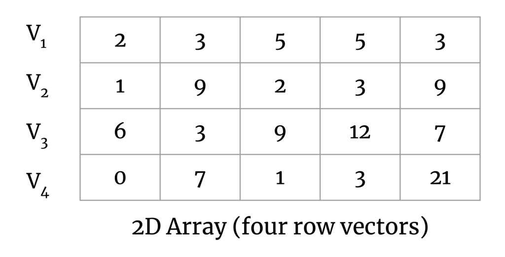
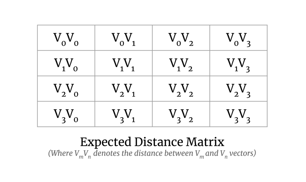
Our goal here is to calculate the pairwise distance between all vector pairs. The output matrix will look like the following:
It solves the problem for smaller datasets and is fast enough, but it doesn’t scale well or utilize GPUs. Therefore, there was a need for a new implementation to handle large datasets and to make use of GPUs.
An implementation with both of these features is available in the sgkit library, and it can be used as follows:
					import dask.array as da
from sgkit.distance.api import pairwise_distance

x = da.random.random((4, 5))
					pairwise_distance(x).compute()

array([[0.        , 0.58320543, 0.85297084, 0.67021758],
       [0.58320543, 0.        , 0.86805965, 0.61936337],
       [0.85297084, 0.86805965, 0.        , 0.78851248],
       [0.67021758, 0.61936337, 0.78851248, 0.        ]])
					pairwise_distance(x, device="gpu").compute()

array([[0.        , 0.58320543, 0.85297084, 0.67021758],
       [0.58320543, 0.        , 0.86805965, 0.61936337],
       [0.85297084, 0.86805965, 0.        , 0.78851248],
       [0.67021758, 0.61936337, 0.78851248, 0.        ]])
To tackle the problem of scaling the computation for large datasets, where the entire array (matrix) would not fit in memory, we took the map-reduce approach on the chunks of the arrays which can be described as follows.
Consider a small chunk of a large 2D array:
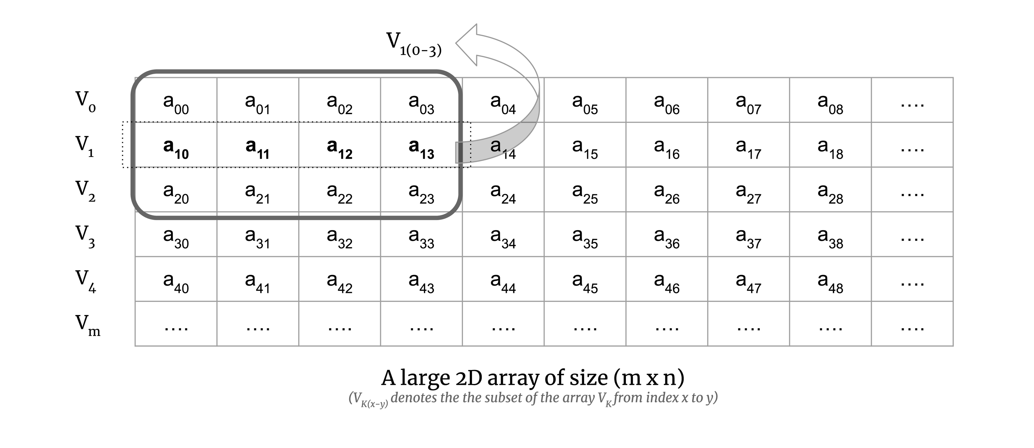
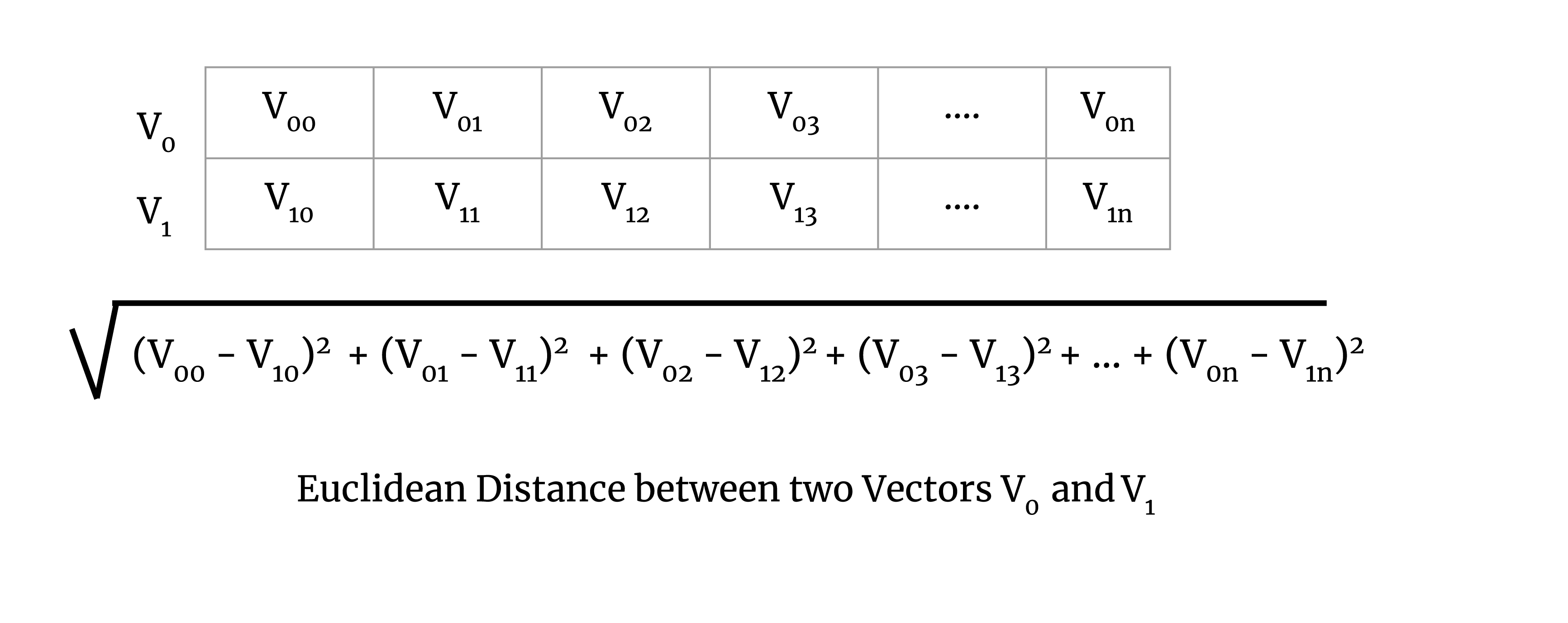
We calculate the map step of the computation on the chunk. To illustrate this, consider Euclidean distance. The Euclidean distance for a pair of vectors V0 and V1 is defined as the square root of
Now to understand map-reduce on a chunk of a large matrix, let’s try to understand it with a simple example of two vectors. To perform the map step of the map-reduce algorithm for Euclidean distance, we calculate the squared sum of a pair of vectors, which is demonstrated in the image below:
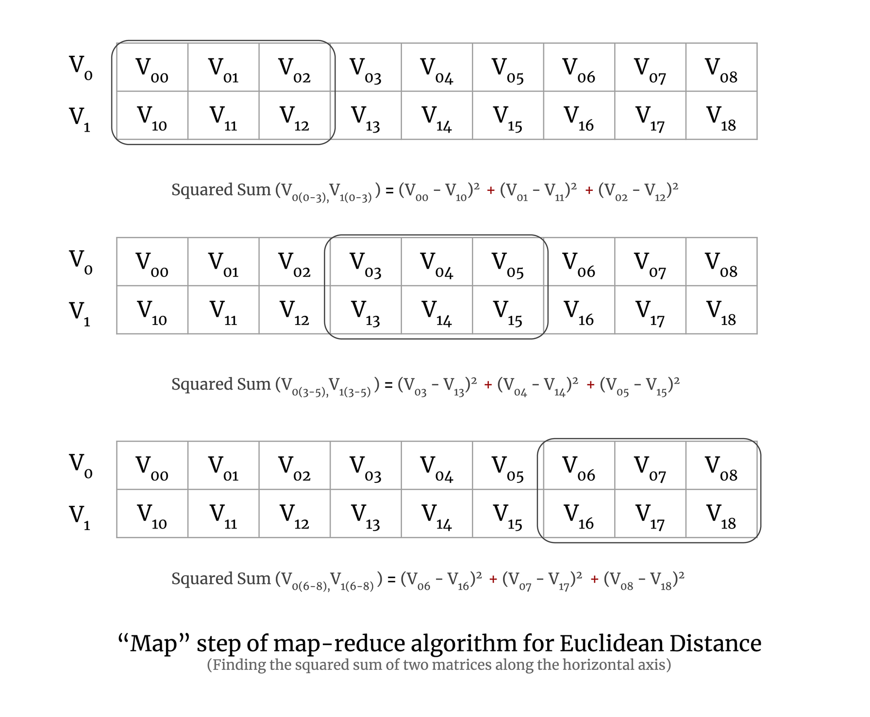
In the above image, you can see that the 2D array has three chunks and we calculate the squared sum for each chunk of the array. In practice, a chunk will have more than two vectors, but here we have taken only two vectors for simplicity.
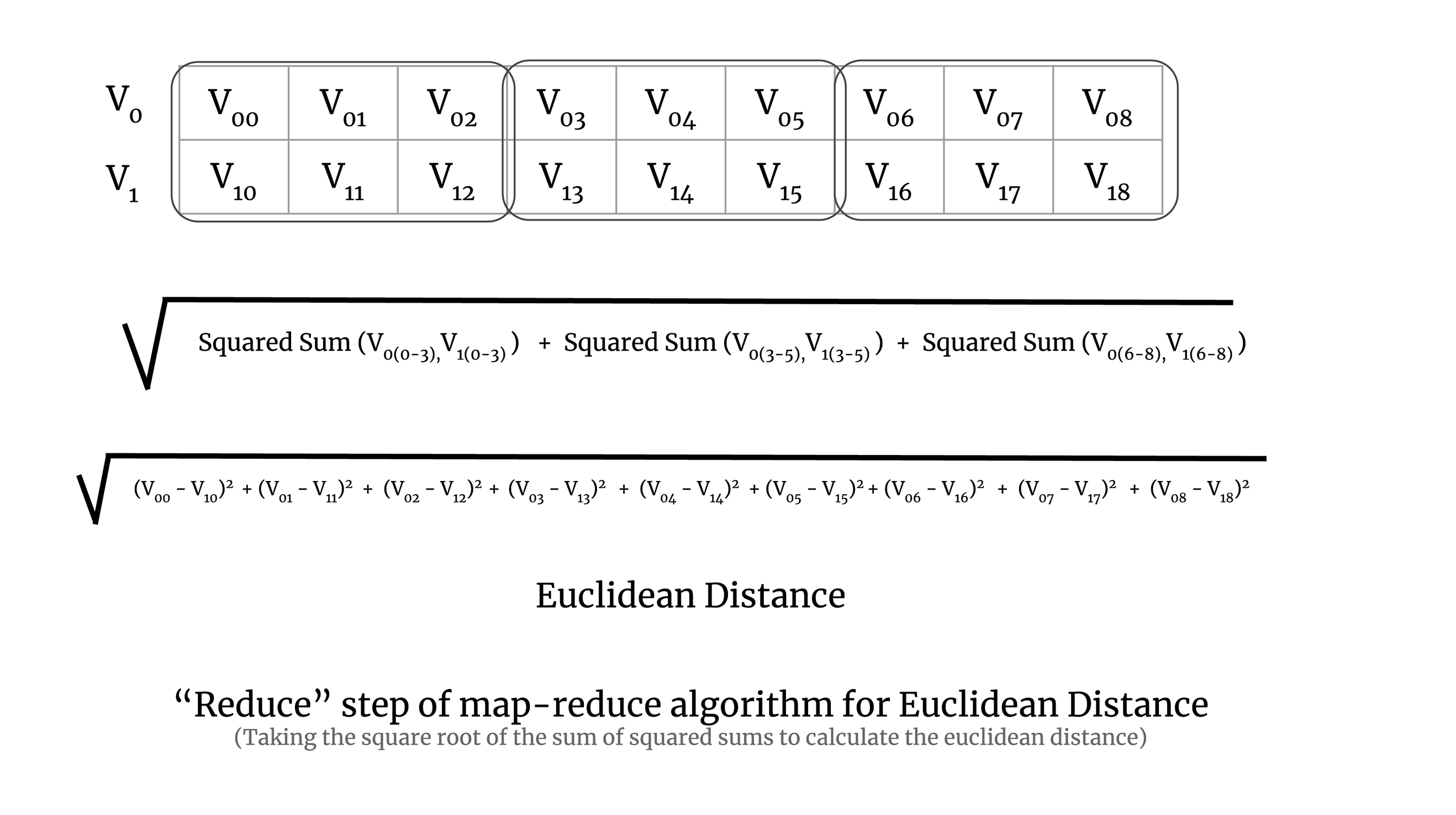
In the reduction step, we take the square root of the sum of all the squared sums of all the chunks. It is demonstrated in the image below:
The implementation was done using Dask and Numba. Dask arrays da.blockwise and da.reduction were used for scaling the map-reduce algorithm to large datasets and Numba’s guvectorize and cuda modules were used for implementing the distance metric map and reduce functions on CPU and GPU. The full implementation of the pairwise distance calculation can be seen in the sgkit source code.
Coiled was used for testing the scalability of the implementation on large datasets and on both CPUs and GPUs.
Here is how one can quickly create a Dask cluster with GPUs on Coiled:
					import coiled
from dask.distributed import Client, performance_report, get_task_stream

account = "aktech"
env_name = f"{account}/sgkit"

coiled.create_software_environment(
    name=env_name,
    conda="environment.yml",
    container="gpuci/miniconda-cuda:10.2-runtime-ubuntu18.04",
)
2. Create cluster configuration for Dask to spin up on Coiled
This will define the name of the cluster configuration and spec for the machine used for a single machine in the cluster. Here we have chosen the machine with 15 GiB RAM, 4 vCPUs, and 1 GPU attached to it.
					coiled.create_cluster_configuration(
    name=env_name,
    software=env_name,
    worker_cpu=4,
    worker_gpu=1,
    worker_memory="15 GiB"
)
3. Create the Dask cluster on Coiled
This will create a Dask cluster with 25 workers and 2 threads each with the dask_cuda.CUDAWorker worker class to handle GPUs.
					cluster = coiled.Cluster(
    configuration=env_name,
    n_workers=25,
    worker_options={"nthreads": 2},
    worker_gpu=1,
    account=account,
    worker_class="dask_cuda.CUDAWorker",
    backend_options={"region": "us-east-1", "spot": False},
)
client = Client(cluster)
print("Dashboard:", client.dashboard_link)
This will also give you the link to the Dask dashboard to see the status of the task.
The dataset used for studying the scalability is the genomic data by MalariaGEN.
Here is the code to run the computation on the MalariaGEN dataset:
					import dask.array as da
import fsspec
import zarr
from dask.distributed import Client
from sgkit.distance.api import pairwise_distance

store = fsspec.get_mapper(
    "gs://ag1000g-release/phase2.AR1/variation/main/zarr/all/ag1000g.phase2.ar1"
)
callset_snps = zarr.open_consolidated(store=store)
gt = callset_snps["2R/calldata/GT"]

gt_da = da.from_zarr(gt)
x = gt_da[:, :, 1].T
x = x.rechunk((-1, 100000))


def run_with_report(x, metric, target, report_name):
    with performance_report(
        filename=f"dask-report-{metric}-{report_name}.html"
    ), get_task_stream(filename=f"task-stream-{metric}-{report_name}.html"):
        out = pairwise_distance(x, metric=metric, target=target)
        out.compute()
Run the computation for the Euclidean metric on GPU on Coiled as follows:
run_with_report(x, metric="euclidean", target="gpu", report_name="full")
Here is a sample output for a small, random matrix, to give an idea of the result of a typical calculation:
					import dask.array as da
from sgkit.distance.api import pairwise_distance

# Create a 5x4 random 2D array to calculate pairwise distance
rs = da.random.RandomState(0)
x = rs.randint(0, 3, size=(5, 4))

# Compute pairwise distance on CPU
pairwise_distance(x).compute()

# Compute pairwise distance on GPU (if you have one)
pairwise_distance(x, device="gpu").compute()
Output:
					array([[0.        , 1.73205081, 2.44948974, 2.23606798, 2.44948974],
       [1.73205081, 0.        , 2.23606798, 2.        , 1.73205081],
       [2.44948974, 2.23606798, 0.        , 1.73205081, 2.44948974],
       [2.23606798, 2.        , 1.73205081, 0.        , 2.23606798],
       [2.44948974, 1.73205081, 2.44948974, 2.23606798, 0.        ]])
In this blog post, we learned how a complex problem of genomics analysis can use Dask to scale to a large dataset and the compute can be easily obtained from Coiled for CPU as well as GPU architectures with just a few lines of code.
The main takeaway here is, if you have a computation that uses Dask and you need compute at scale to speed up the computation, then using Coiled is a very easy way to get compute quickly.