Since 2019 we’ve collaborated with Meta’s PyTorch team and we’re honored to have made direct contributions to a project underlying so many of the generative AI tools emerging daily. See our 2021 and 2022 PyTorch contributions blog posts for more information on our past work.
In this post, we’ll describe some new kernels that Quansight engineers have implemented for block sparse row matrix multiplication involving specific combinations of sparse and dense arguments. These implementations, available in PyTorch 2.1, offer a significant performance improvement over those available in previous versions of PyTorch. We demonstrate these improvements here via some benchmarking results.
Note: We offer PyTorch support as part of our consulting services offerings, so if you’re working with PyTorch and could use some assistance, please take a look at our PyTorch Services page.
Now let’s get to the details.
PyTorch implements a total of 5 sparse layouts. Each layout has properties which make it more, or less, suitable for a particular task. As an example, the coordinate format (COO) can be used to incrementally build sparse tensors, with features that allow individual element access and updates to be more efficient. However, for most mathematical operations, compressed layouts like ‘compressed sparse row’ (CSR) are a better choice since they store specified elements with a more regular structure. This is what a PyTorch tensor looks like using the CSR layout:
					>>> mat = torch.tensor([
    [0, 0, 1, 0, 0, 0],
    [1, 0, 1, 0, 1, 0],
    [0, 0, 0, 1, 0, 0],
    [0, 0, 0, 0, 0, 0],
    [1, 1, 0, 0, 1, 0],
    [0, 0, 0, 0, 0, 0],
])
>>> mat.to_sparse_csr()
tensor(crow_indices=tensor([0, 1, 4, 5, 5, 8, 8]),
       col_indices=tensor([2, 0, 2, 4, 3, 0, 1, 4]),
       values=tensor([1, 1, 1, 1, 1, 1, 1, 1]),
       size=(6, 6),
       nnz=8,
       layout=torch.sparse_csr)
The block sparse row (BSR) layout is closely related to CSR, except that blocks of values are stored instead of single values. This affords many of the same advantages as the CSR layout, with the additional feature that we can use vectorized instructions inside kernels that operate on these block-wise stored values. We can see the clear similarity between the two formats by recasting the example above into the BSR layout:
					>>> mat.to_sparse_bsr((2, 2))
tensor(crow_indices=tensor([0, 3, 4, 6]),
       col_indices=tensor([0, 1, 2, 1, 0, 2]),
       values=tensor([[[0, 0],
                       [1, 0]],
                        ...
                      [[1, 0],
                       [0, 0]]]),
      size=(6, 6), nnz=6, layout=torch.sparse_bsr)
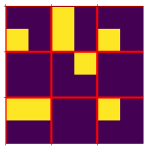
There are some drawbacks to a block sparse layout; a key disadvantage is that we must fully materialize a block if any value within it is non-zero. Larger blocks are generally better for vectorized operations, but may lead to more zero-valued elements being stored. The example we have used here demonstrates this well. In the figure below, we have this matrix with non-zero values in yellow, and the 2×2 block size shown with the red grid. The large number of red blocks that contain mostly zero values illustrates how BSR is less memory efficient for this matrix.
In PyTorch, dense matrix multiplication in eager mode will usually forward to a high performance math library (e.g., cuBLAS) that implements the general matrix multiply (or GEMM) interface. Once we start to involve sparse tensors, though, the situation becomes more complex. We must have a different GEMM-like operation for every pattern of sparse/dense arguments. Here we will focus on two forms involving exactly one sparse argument:
C(Dense) += A(Sparse) @ B(Dense) or DSDC(Sparse) += A(Dense) @ B(Dense) or SDDThe @ symbol is used here to represent the matrix multiplication operation.
The DSD pattern is an operation with the same semantics as a dense matrix multiplication. If the sparse argument were converted to dense, or all implicit zeros were materialized, the result should be equivalent. The DSD pattern can be used to compute linear layers with sparse weights. This is a function which is semantically equivalent to F.linear:
def linear(x, W, b=None):
    tmp = (W @ x.mT).mT
    if b is not None:
        return tmp + b
    else:
        return tmp
In this case, the weights W can be stored using a BSR layout, making this a DSD matrix multiply. Note that linear is defined by x@W^T and above we have calculated the transpose of this expression.
In contrast, the SDD pattern is not semantically equivalent to the dense-to-dense GEMM. In this case, the sparse tensor that is to be updated with the result of A@B also acts as a mask. In other words, C will keep its sparsity pattern, and this will be imposed on the result of A@B. In PyTorch, we call this operation torch.sparse.sampled_addmm. This operation is particularly relevant for transformer models. It can be used to compute masked gradients for terms like linear, where we want to ensure that the sparsity pattern of W is preserved during training.
There exist BLAS-like libraries supporting sparse layouts, for example NVIDIA’s cuSPARSE, and Intel’s MKL sparse API. These libraries are missing features which are required for machine learning applications. First, they typically perform poorly compared to dense matrix multiply except when the sparsity is very high (<10% of the elements are specified). Second, many of the operations are missing support for half-precision data types, which is a feature used frequently in learning applications.
In order to overcome the limitations, we have explored using the Triton language to author kernels, similar to how torch.compile does. We now have prototype implementations available in PyTorch 2.1 for DSD and SDD matrix multiplication using the BSR layout.
We have evaluated the performance of the new DSD and SDD kernels by measuring the speedup compared to the dense implementation. Whenever comparable functionality exists in both PyTorch 2.1 and 2.0, we also compare against the older sparse kernel. All experiments were performed on a single NVIDIA A100-80G GPU, using CUDA 11.8. We evaluated kernels using 2-dimensional tensors with shape (4096,4096) for all tensor arguments. We report performance at different sparsity (%). This metric describes the fraction of elements which are implicitly zero, so a tensor with 90% sparsity contains only 10% of the values compared to a dense tensor with the same shape.
A key detail on the benchmark results figures below is the sparsity ratio (horizontal axis) where the speedup (vertical axis) crosses the 1.0 threshold, which is marked with a horizontal line labeled “1x”. At this point the sparse operation executes faster than the dense baseline. This quantity tells us how much we need to prune to use sparsity without regressing performance.
sampled_addmm (SDD)Strictly speaking, a dense equivalent of sampled_addmm would involve the composition between matrix multiplication and a masking operation. Here, we have chosen for the dense baseline a normal matrix multiplication without masking since, in practice, the masking operation may not be used if the inputs are not sparse (for example, when computing gradients). This gives us a harder target to hit, but is a fair assessment. Looking at the results for the float32 data type, we see some promising results:
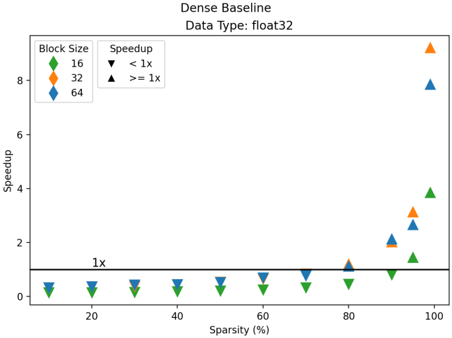
Using block sizes of 32 and 64, we cross the 1x threshold at 80% sparsity. However, the smallest block size of 16 requires 90% sparsity to pass 1x. The small block size is important as it offers more flexibility in the pruning stage: it allows your pruning strategy to more effectively align with the real-world distribution pattern of non-zero elements in your tensor.
Moving on to half-precision data types, we see much poorer performance compared to dense, with the 1x threshold crossed only at 99% sparsity, and only for block sizes of 32 and 64 with the float16 type and a block size of 64 for the bfloat16 type. Requiring pruning to this degree is not practical, as in most cases it will result in unacceptable drops in accuracy.
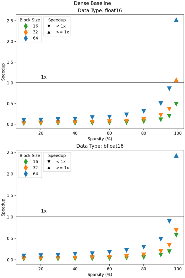
These results, albeit promising, show there is still room for improvement. Support for sampled_addmm is a new feature for BSR layout, and it will continue to improve as we work to make sparsity a practical technique for transformer acceleration.
Note: Although cuSPARSE has added better support for this operation with BSR layout in CUDA 12, we do not expose that interface in PyTorch yet.
bsr_dense_addmm (DSD)The DSD pattern has a direct translation to a dense matrix multiply, so here the experimental setup does not require as much explanation. However, support for this type of sparse-dense matrix multiplication already exists within PyTorch. In PyTorch 2.0 BSR @ Dense multiplication would forward to cuSPARSE for float32, and to a custom implementation for half-precision types. Here we compare to both the dense baseline and these older implementations of the same operation.
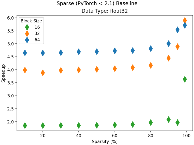
Again, we will look at the performance for float32 first. The plot below compares the new Triton-based implementation to the one available in older versions of PyTorch. The Triton-backed kernels show significant improvements over the previous version. Speedup is fairly constant across sparsity levels at approximately 1.75x, 4.0x, and 4.75x for block size 16, 32, and 64 respectively. There is a sharp rise in the relative performance at very high sparsity. This is a leap forward in terms of raw sparse performance, but we are primarily concerned with performance compared to the dense baseline as this will determine if sparsity can be used without a performance penalty.
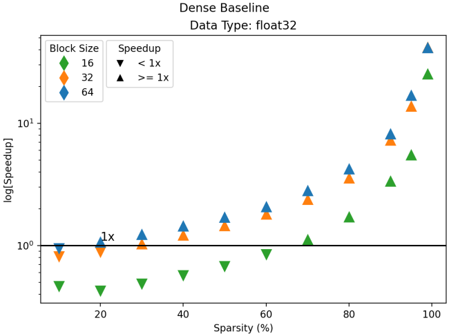
Comparison to the dense baseline is also very promising, as shown in the next figure. Block sizes of 32 and 64 are faster than dense for almost all sparsity ratios, with block size 16 crossing the 1x boundary at 70% sparsity. Further, the float32 performance relative to the dense baseline for larger block sizes is starting to approach ideal behavior. In the ideal situation we could expect the sparse kernel to compute the result with a speedup proportional to the inverse of the sparsity; at 80% sparsity only 1/5 of the tensor values are specified and it should run about 5x faster. This is only possible when the sparse kernel suffers no overhead from metadata lookups. We are very close to this mark with ~3.5x and ~4.5x, for block size 32 and 64, respectively.
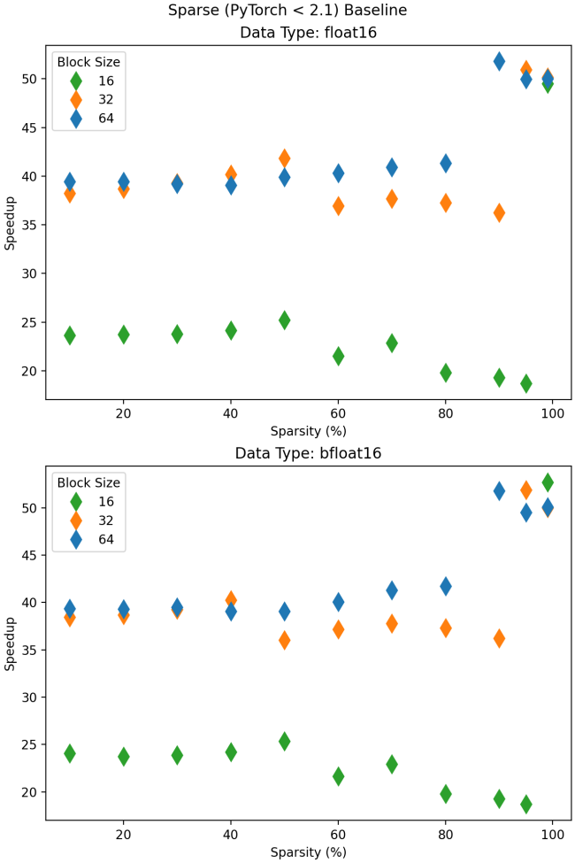
Now we look at the performance for half-precision data types. As shown below, the new kernel provides between 20-50x speedup over the older sparse implementation. While a speedup of this size is still a notable result, cuSPARSE did not natively support half-precision data types, so we knew our previous implementation wasn’t optimal. Instead, it called the dense kernel in a loop for each sparse block which meant each kernel didn’t provide enough work to saturate the GPU, and we suffered the overhead of launching many CUDA kernels.
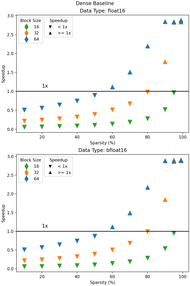
Comparing performance for half-precision types to the dense baseline, we see a clear win. Using a block size of 64, the Triton implementation begins to outperform the dense matrix multiply at 60% sparsity. Unfortunately, this does not hold for smaller block sizes, with 32 reaching >1x speedup above 80% sparsity, and block size 16 only passing this point above 90%.
We are encouraged by these results, but there is more work to do. In particular, performance for half-precision data types is lagging behind. Significant engineering efforts have gone into making the cuBLAS dense matrix multiplication optimized for this case. Our team is up to the challenge, and will continue to close the gap for the sparse kernels provided by PyTorch!
These kernels are not yet considered stable, and only some of the functionality is available through PyTorch operators. They can all be found in the torch.sparse._triton_ops private submodule, for the curious user who wants to experiment with these tools.
If you want to stick to the public features only, the bsr_dense_mm kernel is also fully integrated with matrix multiply ops like torch.mm and torch.addmm. If you meet the following conditions, the work will be forwarded to the Triton kernel:
A in A@B, torch.mm(A, B), or torch.addmm(C, A, B)) has BSR layout, and the other tensors are dense.cuda.torch.float16 or torch.bfloat16.We have made some serious improvements to the usability of key features for BSR, but we are not quite finished yet. These are only the first steps toward a larger goal, namely, making block sparse layouts a first class technique for accelerating transformer workflows. With PyTorch 2.1 coming out, it is a good time to take stock of where we are at, and though we have come a long way, there is plenty of work left to do. We hope to improve on these kernels and add more in the upcoming months. We are also working to enable pathways such that masking behavior for gradients can be accessed without writing a custom autograd function or module.
This work would not have been possible without the close collaboration between Quansight and Meta within the PyTorch project. We thank Christian Puhrsch, Alban Desmaison, and Driss Guessous for their advice and feedback during research and implementation, and their continued support moving forward.
As we noted above, in addition to contributing directly to PyTorch, Quansight also provides support services to assist clients with their use of PyTorch. Check out our PyTorch Support page or reach out to us for more information.